Midpoint Rule Arc Length Calculator
Approximate any curve length with midpoint rectangles and live error checks.
Use x as the variable. Supports +, -, *, /, ^, sqrt, abs, sin, cos, tan, asin, acos, atan, sinh, cosh, tanh, exp, ln, log, pi, e. Examples: 2x means 2*x, x^2 means x squared.
Derivative: automatic (dual numbers)
Derivatives x'(t) and y'(t) are calculated automatically (dual numbers). Use t as the parameter.
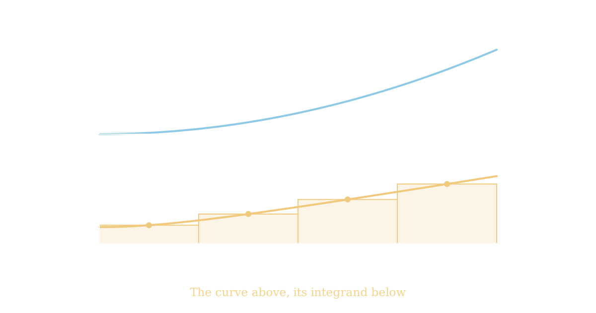
Original Curve & Selected Arc
Gold dots mark the midpoint of each subinterval.
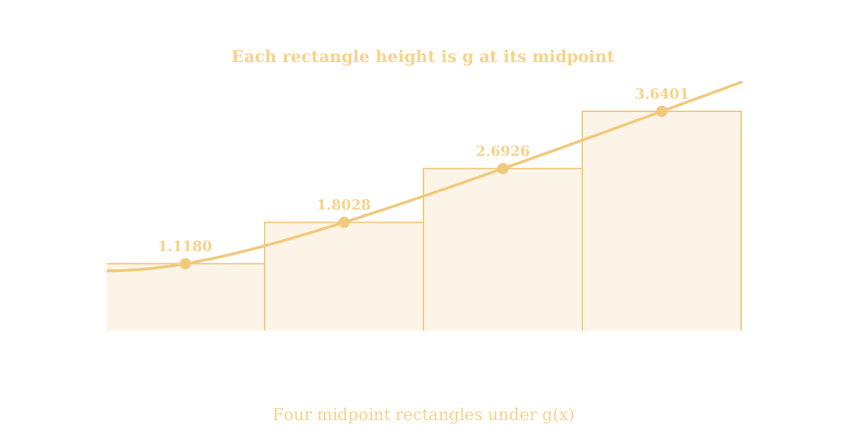
Integrand g(x) & Midpoint Rectangles
Hover a rectangle for its subinterval, midpoint, integrand value and contribution.
Detailed Midpoint Calculation Table
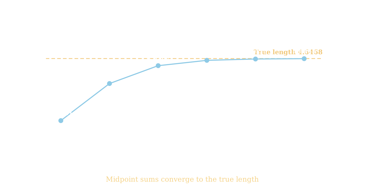
Convergence Comparison
Differences between successive refinements are a practical error indicator, not a guaranteed error bound.
Calculation Error
Section Navigation
How to Use the Midpoint Rule Arc Length Calculator
The Midpoint Rule Arc Length Calculator approximates the length of a curve by dividing the arc-length integral into rectangles and sampling each one at its centre. Enter a function, pick an interval, choose how many subintervals to use, and the calculator shows the approximation, the full midpoint table, the error estimate, and a live diagram of the rectangles. Follow these steps to get a correct answer.
- Choose the calculation mode. Use Explicit Function for a curve written as y = f(x), such as y = x2 or y = sin(x). Use Parametric Curve for a curve written as x = x(t) and y = y(t), such as a circle or an ellipse traced by a parameter.
- Enter the function. Type the function in the input box, using ^ for powers, the square-root function for square roots, and sin(), cos(), exp(), and ln() for the standard functions. The calculator finds the derivative automatically, or you can type the derivative yourself if you already know it.
- Set the interval. Enter the lower limit a and the upper limit b. The interval [a, b] is the stretch of the curve whose length you want. If you enter b smaller than a, the calculator still returns a positive length, because arc length is never negative.
- Choose the number of subintervals n. Use the slider or type a value. Presets include 1, 2, 4, 5, 8, 10, 20, 50, 100, 500, 1,000, and 5,000. A larger n means narrower rectangles and usually a closer approximation. Start with n = 4 to see the working clearly, then raise n to watch the answer settle.
- Pick the display precision. Choose 2, 4, 6, 8, or 10 decimal places. The calculator keeps full precision internally and rounds only the displayed result, so changing the precision never changes the underlying calculation.
- Click Calculate Arc Length. The main result is the midpoint approximation Ln, clearly labelled as an approximation. Below it you get the subinterval width, the first and last midpoints, the first and last integrand values, the sum of the integrand values, the chord length between the endpoints, the high-accuracy reference length, and the estimated absolute and relative errors.
- Study the diagrams. The first diagram shows the original curve with the selected arc highlighted and the midpoint sample points marked. The second diagram shows the arc-length integrand with the midpoint rectangles drawn under it. The total area of those rectangles is the approximation, so the two diagrams must not be confused: the rectangles belong under the integrand, never under the original curve.
- Read the calculation table. Every subinterval gets a row with its boundaries, its midpoint, the derivative at the midpoint, the integrand value, and the rectangle contribution. The final row shows the sum, which equals the main result.
- Compare convergence and try Richardson extrapolation. The convergence panel shows the approximations for n, 2n, and 4n side by side, with the differences between them. The Richardson option combines two approximations into a refined estimate. Both are explained in the guide sections below.
- Copy, export, or reset. Use Copy Result for the answer, export the table as CSV for your working, or Reset to clear the panel. The preset buttons load verified examples instantly: the parabola, the straight line, the horizontal line, the quarter circle, the cubic, and the sine curve.
Try an example. y = x2 on [0, 2] with n = 4 gives L4 = 4.6267234873 units, against a reference of 4.6467837624 units. y = 3x + 1 on [0, 4] with n = 4 gives exactly 12.6491106407 units. y = 2 on [1, 5] with n = 4 gives exactly 4.0000000000 units. The parametric quarter circle of radius 5 gives 7.8539816340 units. y = x3 on [0, 1] with n = 4 gives 1.5330289642 units, and y = sin(x) on [0, π] with n = 8 gives 3.8201978627 units.
Important tips. Always differentiate the function first: the integrand uses f'(x), not f(x). Sample at midpoints, not at endpoints, or you are computing a different rule. Keep the angle unit in radians for trigonometric functions. Do not round the midpoints or the integrand values mid-calculation, because those small roundings add up across many rectangles. If the function is undefined at a midpoint, the calculator reports an error instead of silently skipping the sample.
What Is the Midpoint Rule?
Numerical integration is the art of estimating a definite integral when an exact antiderivative is hard to find, or when only sampled values are available. The midpoint rule is one of the simplest and most reliable numerical integration methods. It estimates the area under a curve by covering it with rectangles and adding up their areas.
A Riemann sum divides the interval [a, b] into n equal subintervals, each of width Δx = (b - a) / n, and builds one rectangle on each subinterval. The height of each rectangle is the value of the function at a single sample point inside that subinterval. Left-endpoint sums sample at the left edge, right-endpoint sums sample at the right edge, and the midpoint rule samples at the centre of each subinterval.
Sampling at the centre is the key idea. On a short subinterval, a curve that rises on one side of the midpoint falls on the other side by a similar amount, so the overestimate on one half roughly cancels the underestimate on the other half. That cancellation is why the midpoint rule is more accurate than the left or right endpoint rules with the same number of rectangles, and why its error shrinks with the square of the subinterval width.
For a function g(x) on [a, b], the composite midpoint rule is:
Here xi* is the midpoint of the ith subinterval, and the sum runs over all n subintervals. Each term Δx × g(xi*) is the area of one rectangle, and the sum of all the rectangle areas is the approximation of the integral.
The midpoint rule is used far beyond calculus homework. Engineers use it to estimate integrals in stress analysis and signal processing, physicists use it in numerical simulations, and computer graphics uses it to measure curve lengths and surface areas. Its combination of simplicity and second-order accuracy makes it a standard first choice whenever an integral has no tidy closed form.
Why midpoints beat endpoints. Take g(x) = x on [0, 1] with n = 1. The left sum gives 0, the right sum gives 1, and the midpoint sum gives 0.5, which is the exact answer. The midpoint sees the average behaviour of the function across the subinterval, while an endpoint sees only one side of it. That advantage holds for any smooth function, and it is the reason the midpoint rule is the default Riemann sum in most numerical work.
What Is Arc Length?
Arc length is the distance measured along a curve, rather than the straight-line distance between its endpoints. A road that winds through hills is longer than the straight line drawn between its two ends on a map. A curved wire is longer than the gap it spans. Arc length measures the winding path itself.
To find that length, imagine cutting the curve into many tiny pieces. Each tiny piece is so short that it is almost straight, so its length is close to the straight line joining its ends. By the Pythagorean theorem, a tiny piece that moves Δx horizontally and Δy vertically has length close to √(Δx2 + Δy2). Adding up all the tiny pieces gives the total length, and letting the pieces shrink to zero turns the sum into an integral.
For a curve y = f(x), a tiny horizontal step dx produces a vertical change dy = f'(x) dx, so the tiny length element is:
Adding up all the length elements from a to b gives the arc-length integral:
That formula explains why the derivative is involved. A steep curve changes height fast, so f'(x) is large, the integrand √(1 + [f'(x)]2) is large, and each unit of horizontal distance contributes more than one unit of curve length. A flat curve has f'(x) close to zero, the integrand is close to 1, and the arc length is close to the horizontal distance b - a.
Arc length is always at least as long as the chord. The straight line between the endpoints is the shortest path between them, so the curve can never be shorter than it. For the parabola y = x2 on [0, 2], the chord from (0, 0) to (2, 4) is √(20) = 4.4721359550 units, while the true arc length is 4.6467837624 units, longer by 0.1746478074 units. For the sine curve y = sin(x) on [0, π], the chord is π = 3.1415926536 units and the arc is 3.8201977890 units, longer by 0.6786051354 units. Checking that the arc exceeds the chord is a quick sanity test for any arc-length answer.
Most arc-length integrals have no elementary antiderivative. The parabola integral ∫ √(1 + 4x2) dx can be done with a substitution, but the sine integral ∫ √(1 + cos2x) dx cannot be expressed with elementary functions at all. That is exactly where the midpoint rule earns its place: it estimates the integral numerically, without needing an antiderivative.
Midpoint Rule Arc Length Formula
The midpoint rule arc-length calculation starts from the exact arc-length integral and replaces the integral with a sum of rectangle areas. Define the arc-length integrand:
Then the exact arc length is L = ∫ab g(x) dx, and the midpoint rule approximates that integral. Divide [a, b] into n equal subintervals. The subinterval width is:
The midpoint of the ith subinterval, counting i from 0, is:
Evaluate the integrand at each midpoint, multiply each value by Δx, and add the results:
Each symbol has a precise meaning:
| Symbol | Meaning | Notes |
|---|---|---|
| L | Exact arc length | The true curved distance, usually unknown |
| Ln | Midpoint approximation | The calculator's main result for n subintervals |
| f(x) | The function | The curve whose length is measured |
| f'(x) | First derivative | The slope of the curve at x |
| g(x) | Arc-length integrand | g(x) = √(1 + [f'(x)]2) |
| a, b | Integration limits | Lower and upper ends of the interval |
| n | Number of subintervals | More subintervals usually means a closer answer |
| Δx | Subinterval width | Δx = (b - a) / n |
| xi* | Midpoint of subinterval i | xi* = a + (i + ½)Δx |
A concrete check. For y = x2 on [0, 2] with n = 4, the width is Δx = (2 - 0) / 4 = 0.5, the midpoints are 0.25, 0.75, 1.25, and 1.75, and the integrand values are 1.1180339887, 1.8027756377, 2.6925824036, and 3.6400549446. Their sum is 9.2534469747, and multiplying by 0.5 gives L4 = 4.6267234873 units. Every number in that chain is shown in the calculator's step-by-step panel and in its calculation table.
For a parametric curve x = x(t), y = y(t), the same idea applies to the parameter interval [t1, t2], with the speed v(t) = √([x'(t)]2 + [y'(t)]2) playing the role of the integrand. The parametric formula is covered in its own section below.
How to Calculate Arc Length Using the Midpoint Rule
The midpoint rule calculation follows ten steps, and the calculator performs all of them automatically. Working through them by hand once makes the tool far easier to trust and to use. The worked example below uses y = x2 on [0, 2] with n = 4, the same example the calculator loads as its first preset.
- Identify the function. f(x) = x2.
- Find its first derivative. f'(x) = 2x.
- Identify the integration interval. a = 0, b = 2.
- Choose the number of subintervals. n = 4.
- Calculate the subinterval width. Δx = (2 - 0) / 4 = 0.5.
- Determine the midpoint of each subinterval. x0* = 0.25, x1* = 0.75, x2* = 1.25, x3* = 1.75. Each midpoint sits exactly halfway between its subinterval boundaries: 0.25 is halfway between 0 and 0.5, 0.75 is halfway between 0.5 and 1, and so on.
- Evaluate the arc-length integrand at each midpoint. g(x) = √(1 + 4x2), so g(0.25) = 1.1180339887, g(0.75) = 1.8027756377, g(1.25) = 2.6925824036, and g(1.75) = 3.6400549446.
- Multiply each value by the subinterval width. The four rectangle contributions are 0.5 × 1.1180339887 = 0.5590169944, 0.5 × 1.8027756377 = 0.9013878189, 0.5 × 2.6925824036 = 1.3462912018, and 0.5 × 3.6400549446 = 1.8200274723.
- Add all contributions. 0.5590169944 + 0.9013878189 + 1.3462912018 + 1.8200274723 = 4.6267234873.
- Interpret the approximate arc length. L4 = 4.6267234873 units. The high-accuracy reference is 4.6467837624 units, so this approximation is short by 0.0200602751 units, a relative error of 0.4317%.
The same ten steps work for any function. For y = x3 on [0, 1] with n = 4, the derivative is f'(x) = 3x2, the width is Δx = 0.25, the midpoints are 0.125, 0.375, 0.625, and 0.875, the integrand values are 1.0010980300, 1.0853471867, 1.5405489332, and 2.5051217067, their sum is 6.1321158566, and multiplying by 0.25 gives L4 = 1.5330289642 units, against a reference of 1.5478656547 units.
A second worked example with a trigonometric function. For y = sin(x) on [0, π] with n = 8, the derivative is f'(x) = cos(x), the width is Δx = π / 8 = 0.3926990817, and the eight midpoints are π/16, 3π/16, 5π/16, 7π/16, 9π/16, 11π/16, 13π/16, and 15π/16. The integrand values, in order, are 1.4006926023, 1.3005159423, 1.1439660326, 1.0188524102, 1.0188524102, 1.1439660326, 1.3005159423, and 1.4006926023. Their sum is 9.7280539749, and multiplying by 0.3926990817 gives L8 = 3.8201978627 units, against a reference of 3.8201977890 units, an absolute error of only 0.0000000736 units.
Understanding Midpoint Rectangles
Each midpoint rectangle is a small, honest picture of one piece of the integral. It has three parts, and each part has a clear meaning.
| Rectangle part | Formula | Meaning |
|---|---|---|
| Width | Δx = (b - a) / n | The horizontal span of one subinterval |
| Height | g(xi*) | The integrand value at the subinterval midpoint |
| Area | Δx × g(xi*) | The contribution of that subinterval to the total |
For the parabola y = x2 on [0, 2] with n = 4, the four rectangles all have width 0.5. Their heights are 1.1180339887, 1.8027756377, 2.6925824036, and 3.6400549446, and their areas are 0.5590169944, 0.9013878189, 1.3462912018, and 1.8200274723. The total area is 4.6267234873 units, which is exactly the midpoint approximation L4.
Why the sum of the areas approximates the integral. The integral ∫ab g(x) dx is the exact area under the integrand curve. Each rectangle replaces the curved strip above one subinterval with a flat-topped strip of the same width, using the midpoint height as the representative height. Where the integrand curves upward, the flat top cuts off a little area on one side and adds a little on the other. Because the sample is taken at the centre, those two errors nearly cancel, and the rectangle area is close to the true strip area. Adding the rectangles gives an estimate of the whole area, and therefore of the arc length.
The most common diagram mistake. The rectangles must be drawn under the integrand curve g(x) = √(1 + [f'(x)]2), not under the original curve f(x). The original curve and the integrand are different graphs with different heights: for y = x2 on [0, 2], the original curve runs from 0 to 4, while the integrand runs from 1 to √(17) = 4.1231056256. Rectangles drawn under the original curve would sum to the area under f(x), which has nothing to do with arc length. The calculator keeps the two graphs separate, and the guide diagram above shows the rectangles under the integrand only.
Reading a rectangle. Hovering over or selecting a rectangle in the calculator shows its subinterval number, its left and right boundaries, its midpoint, the derivative at the midpoint, the integrand value, and the rectangle contribution. That detail is what makes the table useful for homework: every number in the final answer can be traced back to one rectangle.
Why Does the Number of Subintervals Matter?
The number of subintervals n is the single most important control on the calculator, because it decides how fine the rectangles are. A small n means a few wide rectangles. A large n means many narrow rectangles that follow the integrand curve closely.
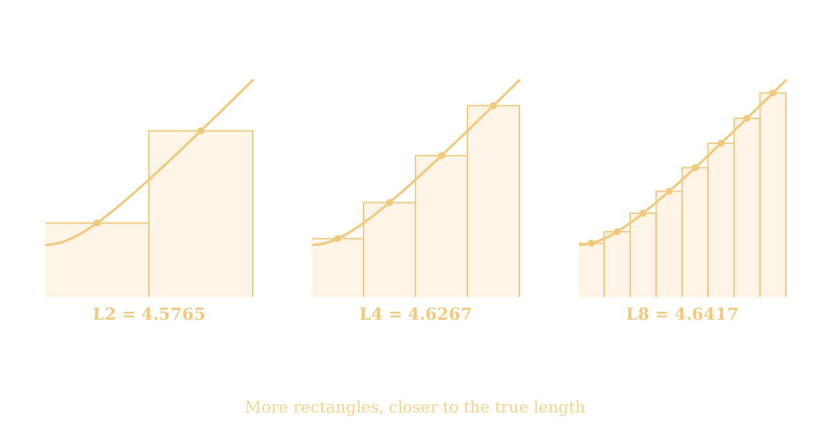
What happens when n is small. With n = 1, the whole interval is one rectangle, and the answer is Δx × g(midpoint). For the parabola y = x2 on [0, 2], n = 1 gives 2 × √(5) = 4.4721359550 units, which is short of the true 4.6467837624 units by 0.1746478074 units. The single rectangle cannot follow the integrand as it rises from 1 to 4.1231056256, so the error is large. With n = 2, the answer improves to 4.5764912225 units. With n = 4, it is 4.6267234873 units. With n = 8, it is 4.6417306581 units. With n = 16, it is 4.6455205322 units, and with n = 32, it is 4.6464679593 units.
How the error shrinks. For a smooth integrand, the midpoint rule error is proportional to 1 / n2. Doubling n cuts the error to roughly one quarter. The parabola numbers show this clearly: the error falls from 0.0200602751 units at n = 4 to 0.0050531044 units at n = 8, then to 0.0012632302 units at n = 16, then to 0.0003158031 units at n = 32. Each doubling divides the error by about four. That 1 / n2 behaviour is called second-order convergence, and it is the reason the midpoint rule is so effective: a modest increase in n buys a large improvement in accuracy.
Why the improvement is not always monotonic. The error usually shrinks as n grows, but it does not have to shrink at every step for every function. The sine curve shows a mild version of this: n = 2 gives 3.8476494905 units, which overshoots the reference 3.8201977890 units, while n = 4 gives 3.8204517876 units, which is much closer. The approximation crossed from above the true value to a value just above it, and the error still shrank overall. For functions with sharp bends, oscillations, or near-singularities, the error can wobble as n changes, even though the long-run trend is downward. Never assume that a larger n always gives a better answer for a single step; check the convergence table instead.
The cost of a larger n. More subintervals mean more arithmetic: more derivative evaluations, more integrand values, and more table rows. For n = 5,000, the calculator performs 5,000 evaluations, which is fast for a computer but produces a table too long to read row by row, so the calculator paginates it. The practical rule is to raise n until the answer stops changing at the precision you need. If n = 100 and n = 200 agree to six decimal places, n = 100 is enough, and n = 5,000 adds nothing but work.
Choosing n in practice. Use n = 4 or n = 8 while learning, because the table stays short enough to check by hand. Use n = 50 or n = 100 for homework answers that need four or five correct decimal places. Use n = 1,000 or more only when you need very high precision, or when the integrand changes quickly over the interval. The convergence panel shows n, 2n, and 4n together, so you can see the answer settling without guessing.
Midpoint Rule vs Trapezoidal Rule vs Simpson's Rule
The midpoint rule is one of three classic numerical integration methods, and each one samples the integrand differently. Knowing how they differ helps you pick the right tool and understand why their answers disagree.
| Feature | Midpoint rule | Trapezoidal rule | Simpson's rule |
|---|---|---|---|
| Sample locations | Midpoint of each subinterval | Both endpoints of each subinterval | Endpoints plus midpoints |
| Shape fitted | Flat-topped rectangle | Straight-sided trapezium | Parabola through three points |
| Error order | O(1 / n2) | O(1 / n2) | O(1 / n4) |
| Typical error sign | Opposite to trapezoidal | Opposite to midpoint | Usually smallest of the three |
| Evaluations needed | n | n + 1 | 2n + 1 |
| Restriction | None | None | n must be even |
| Exact for | Constant and linear functions | Constant and linear functions | Polynomials up to degree 3 |
Midpoint rule. Samples at the centre of each subinterval and builds rectangles. Its error is O(1 / n2), the same order as the trapezoidal rule, but the midpoint rule is usually about twice as accurate as the trapezoidal rule for the same n, because the centre sample cancels the leading error. It needs only n evaluations, one per subinterval, and it works for any positive n.
Trapezoidal rule. Samples at the endpoints and joins them with straight lines, forming trapeziums. It shares the midpoint rule's O(1 / n2) error order, but its error usually has the opposite sign: for a convex integrand, the trapezoidal rule overestimates while the midpoint rule underestimates, or the other way round. Averaging the two gives the trapezoidal-midpoint combination, which is the basis of Simpson's rule. Try the trapezoidal rule calculator to compare the two methods on the same function.
Simpson's rule. Fits a parabola through the two endpoints and the midpoint of each pair of subintervals, which needs an even number of subintervals. Its error is O(1 / n4), so it converges far faster than either of the other two for smooth functions. The price is the even-n restriction and more evaluations per subinterval. Try the Simpson's rule calculator when you need high accuracy with few subintervals.
A number comparison. For the parabola y = x2 on [0, 2] with n = 4, the midpoint rule gives 4.6267234873 units, the trapezoidal rule gives 4.6870560064 units, and Simpson's rule gives 4.6502010785 units, against the reference 4.6467837624 units. The midpoint error is 0.0200602751 units, the trapezoidal error is 0.0402722440 units, and the Simpson error is 0.0034173160 units. Simpson wins here, as it usually does for smooth functions, but the midpoint rule is simpler, needs no even-n restriction, and is the natural choice when only midpoint samples are available.
Which rule should you use? Use the midpoint rule when you want a simple, reliable estimate, when you are sampling a function at evenly spaced interior points, or when you are teaching Riemann sums. Use the trapezoidal rule when endpoint values are the natural data, such as measurements taken at the ends of each interval. Use Simpson's rule when the function is smooth and you need high accuracy with a small n. For arc length specifically, the midpoint rule has a practical advantage: it never evaluates the integrand at the endpoints, where a function can be undefined or singular, so it can handle curves that the other two rules cannot start on.
Understanding Midpoint Rule Error
Every midpoint approximation differs from the true arc length by some amount, and understanding that error is what turns a number into a trustworthy answer. There are three different ways to talk about error, and they must not be confused.
Absolute error. The absolute error is the size of the gap between the approximation and the true value: |L - Ln|. For the parabola with n = 4, the absolute error is |4.6467837624 - 4.6267234873| = 0.0200602751 units. For the sine curve with n = 8, it is |3.8201977890 - 3.8201978627| = 0.0000000736 units. Absolute error is measured in the same units as the length itself.
Relative error. The relative error divides the absolute error by the size of the true value, and is usually given as a percentage: |L - Ln| / |L| × 100. For the parabola with n = 4, the relative error is 0.4317%. For the cubic with n = 4, it is 0.9585%. For the sine curve with n = 8, it is 0.00000193%. Relative error is the fair way to compare accuracy across problems of different sizes: an error of 0.02 units matters little on a length of 100 units and a great deal on a length of 0.1 units.
Refinement-based error indicator. In real work the true value is unknown, so the absolute error cannot be computed directly. Instead, compare two approximations: the difference |M2n - Mn| shows how much the answer moved when the partition was refined. For the parabola, |M8 - M4| = |4.6417306581 - 4.6267234873| = 0.0150071707 units. That difference is a practical warning signal: if it is large, the answer is still moving and n should be raised. It is an indicator, not a guaranteed bound: the true error can be larger or smaller than the refinement difference, and it is usually about one third of it for the midpoint rule, because the error shrinks by a factor of four at each doubling.
Theoretical error bound. For a sufficiently smooth integrand g(x), the composite midpoint rule error satisfies:
The bound needs the maximum of the second derivative of the integrand over the interval, which is often hard to find exactly. For the parabola integrand g(x) = √(1 + 4x2), the second derivative is g''(x) = 4 / (1 + 4x2)3/2, whose largest value on [0, 2] is 4 at x = 0. The bound for n = 4 is therefore (8 / (24 × 16)) × 4 = 0.0833333333 units, and the actual error 0.0200602751 units sits safely inside it. For n = 8, the bound is 0.0208333333 units. The bound is honest but loose: it overestimates the real error by a factor of four here, which is typical.
When the bound does not apply. The error bound assumes the integrand is smooth, with a bounded second derivative. A function with a corner, a jump, or a singularity breaks that assumption, and the bound either does not exist or is uselessly large. The calculator does not invent a bound when it cannot certify one. In that case it shows the refinement difference and explains its limits, which is the honest answer.
Why smoothness matters. The 1 / n2 error behaviour depends on the integrand being smooth enough for the midpoint cancellation to work. A smooth integrand such as √(1 + 4x2) converges cleanly. An integrand with a sharp corner converges more slowly, and an integrand with a singularity may converge very slowly or not at all. If doubling n barely changes the answer, the function may be smooth and already accurate. If doubling n changes the answer a lot, either the function is rough or n is still too small.
What Is Richardson Extrapolation?
Richardson extrapolation is a simple trick that turns two midpoint approximations into one much better estimate. It uses the known pattern of the midpoint rule error to cancel the leading error term.
For a smooth integrand, the midpoint approximation with n subintervals has an error that behaves like C / n2, where C is a constant that depends on the function but not on n. Doubling the subintervals to 2n therefore divides the error by four. That gives two equations in two unknowns, the true value L and the constant C:
Solving for L eliminates C and leaves the Richardson extrapolated estimate:
Worked example. For the parabola y = x2 on [0, 2], M4 = 4.6267234873 units and M8 = 4.6417306581 units. The Richardson estimate is LR = (4 × 4.6417306581 - 4.6267234873) / 3 = 4.6467330483 units. The true value is 4.6467837624 units, so the extrapolated error is only 0.0000507141 units, far smaller than the original M4 error of 0.0200602751 units. The extrapolation bought the accuracy of a much larger n using only the n = 4 and n = 8 calculations.
Worked example with the sine curve. For y = sin(x) on [0, π], M8 = 3.8201978627 units and M16 = 3.8201977890 units. The Richardson estimate is LR = (4 × 3.8201977890 - 3.8201978627) / 3 = 3.8201977645 units, against the reference 3.8201977890 units, an error of only 0.0000000245 units.
Worked example with the cubic. For y = x3 on [0, 1], M4 = 1.5330289642 units and M8 = 1.5441590533 units. The Richardson estimate is LR = (4 × 1.5441590533 - 1.5330289642) / 3 = 1.5478690830 units, against the reference 1.5478656547 units, an error of 0.0000034283 units. The original M4 error was 0.0148366905 units, so the extrapolation cut it by a factor of about 4327.7.
What Richardson extrapolation is not. The extrapolated value is a refined estimate, not the midpoint rule result and not a guaranteed exact answer. It assumes the error really does behave like C / n2, which holds for smooth integrands and fails for rough ones. If the integrand has a corner or a singularity, the extrapolation can be worse than the original approximation, so the calculator always shows the original midpoint result first and labels the extrapolated value separately. Richardson extrapolation is also the idea behind Romberg integration, which repeats the same trick at several levels to reach very high accuracy.
Parametric Arc Length Using the Midpoint Rule
Some curves cannot be written as y = f(x). A circle, for example, gives two y values for most x values, so no single function describes it. Parametric curves solve this by describing both coordinates as functions of a parameter t: x = x(t) and y = y(t). As t runs from t1 to t2, the point (x(t), y(t)) traces the curve.
For a parametric curve, the tiny length element comes from the movement in both coordinates: ds = √(dx2 + dy2). Writing dx = x'(t) dt and dy = y'(t) dt gives the parametric arc-length integral:
The quantity under the square root is the speed v(t) = √([x'(t)]2 + [y'(t)]2), the rate at which the point moves along the curve as t changes. The midpoint rule applies to the parameter interval exactly as it applies to an x interval: divide [t1, t2] into n equal sections of width Δt = (t2 - t1) / n, sample the speed at the midpoint parameters ti* = t1 + (i + ½)Δt, and add the contributions:
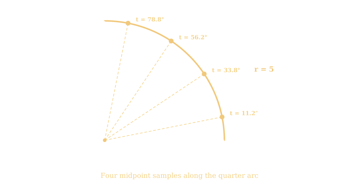
Worked example: the quarter circle. Take x(t) = 5 cos(t) and y(t) = 5 sin(t) on [0, π/2], with n = 4. The derivatives are x'(t) = -5 sin(t) and y'(t) = 5 cos(t). The speed is v(t) = √(25 sin2(t) + 25 cos2(t)) = √(25) = 5, a constant, because sin2(t) + cos2(t) = 1. The parameter width is Δt = (π/2 - 0) / 4 = π/8 = 0.3926990817, and the midpoint parameters are π/16, 3π/16, 5π/16, and 7π/16. Every speed value is 5, so every contribution is 0.3926990817 × 5 = 1.9634954085, and the total is 4 × 1.9634954085 = 7.8539816340 units, which is exactly 5π/2. The midpoint rule is exact here for any n, because the speed is constant.
Why the parametric form matters. Many real curves are naturally parametric: circles, ellipses, spirals, Bezier curves in design software, and the paths of moving objects in physics and robotics. The explicit form y = f(x) cannot describe a curve that doubles back on itself, but the parametric form can. The calculator handles both forms with the same midpoint engine, the same table, and the same convergence analysis. For more on parametric curves, see the parametric arc length calculator.
A warning about the parameter. The parameter t is not the same as arc length unless the speed is 1. Equal steps in t give equal steps along the curve only when the speed is constant. For a general parametric curve, the midpoint rule still works correctly, because it integrates the speed, but the rectangles are equal in t, not equal in distance along the curve. That is fine: the formula accounts for it through v(t).
When Is the Midpoint Rule Useful?
The midpoint rule is useful wherever an integral has to be estimated numerically, and arc length is only one of its jobs. Its simplicity, its second-order accuracy, and its tolerance for endpoint problems make it a workhorse across many fields.
Numerical calculus and education. The midpoint rule is often the first numerical integration method students meet, because rectangles are easy to draw and the midpoint idea is easy to grasp. It teaches Riemann sums, convergence, and error analysis in one package. This calculator's table and diagrams are built for exactly that purpose: every number in the answer can be traced to one rectangle.
Engineering. Engineers estimate lengths of curved parts, cables, pipes, and road bends from mathematical models. When the curve is a polynomial or a trigonometric function, the arc-length integral often has no closed form, so a numerical method is the only option. The midpoint rule gives a fast answer with a clear error estimate, and raising n refines it as far as the design needs.
Physics. Physicists integrate along paths to compute work, distance travelled, and field quantities. A particle moving along a curved path covers a distance equal to the arc length of its trajectory, and the midpoint rule estimates that distance from the velocity data. The same method estimates integrals in thermodynamics, optics, and quantum mechanics, wherever an analytic antiderivative is out of reach.
Computer graphics and CAD. Curves on a screen are drawn as many short straight segments, and the total length of a curve is estimated by adding those segments, which is a form of numerical integration. Font outlines, animation paths, and CAD tool paths all depend on accurate curve-length measurement. The midpoint rule gives a principled way to measure those lengths instead of guessing from a picture.
Curve measurement and robotics. A robot arm moving its gripper along a circular arc, a CNC machine cutting a curved edge, or a surveyor measuring a curved boundary all need the length of a curve that is known only through its equation or through sampled points. The midpoint rule turns those samples into a length, with an error estimate that says how far the answer can be trusted.
Scientific modelling and computational geometry. Models in biology, finance, and climate science integrate functions that are known only at discrete points. The midpoint rule is the natural choice when the data are samples taken at the centres of intervals, which is common in sensor readings and simulation output. In computational geometry, it measures perimeters of curved shapes and lengths of spline curves.
When not to use it. The midpoint rule is a poor choice when the integrand has a singularity inside the interval, when the function is discontinuous, or when very high accuracy is needed with few evaluations: Simpson's rule or an adaptive method will do better there. It is also the wrong tool when the integral itself is not the question, such as when a closed-form arc length is already known. A circle of radius 5 has a quarter-circle arc of exactly 5π/2 = 7.8539816340 units, and no numerical method can improve on that.
Common Mistakes When Using the Midpoint Rule
Most wrong midpoint answers come from a short list of errors. Checking for each one takes seconds and saves most mistakes.
- Using endpoints instead of midpoints. Sampling at the left or right edge of each subinterval computes the left or right Riemann sum, not the midpoint rule. For the parabola y = x2 on [0, 2] with n = 4, the left sum is 3.75 units and the right sum is 5.75 units, while the midpoint rule gives 4.6267234873 units. Only the midpoint value is the midpoint rule answer.
- Forgetting to differentiate the function. The integrand is g(x) = √(1 + [f'(x)]2), not √(1 + [f(x)]2). For y = x2, using f(x) instead of f'(x) gives the integral of √(1 + x4), a different number entirely. Always differentiate first.
- Using the wrong arc-length integrand. The integrand must be √(1 + [f'(x)]2). Dropping the 1, forgetting the square, or taking the square root of the wrong quantity all give wrong answers. For a straight line with slope 3, the integrand is the constant √(10) = 3.1622776602, not 3 and not √(1 + 3).
- Dividing the interval incorrectly. The width is Δx = (b - a) / n, with the full interval length on top. Dividing by n + 1, or using b / n instead of (b - a) / n, shifts every midpoint and corrupts the answer. For [0, 2] with n = 4, the width is 0.5, not 0.4 and not 0.6666666667.
- Using the wrong number of midpoints. There are exactly n midpoints, one per subinterval, not n + 1. The endpoints are not midpoints. Counting n + 1 sample points means one subinterval was counted twice or an endpoint was sampled by mistake.
- Confusing the original curve with the integrand graph. The midpoint rectangles sit under the integrand g(x), not under the original curve f(x). Drawing them under f(x) and adding their areas gives the area under f(x), which is not the arc length. The two graphs are different curves and must be shown separately.
- Rounding intermediate values. Rounding the midpoints, the derivative values, or the integrand values before adding them up introduces small errors that accumulate across many rectangles. Keep full precision through the calculation and round only the final displayed result. The calculator does this automatically.
- Assuming every approximation is exact. The midpoint rule gives an approximation, not the true value, except in special cases such as straight lines and constant-speed parametric curves. For the parabola, L4 = 4.6267234873 units is close to the true 4.6467837624 units, but it is not equal to it. Always report the result as an approximation and give the error estimate alongside it.
- Confusing estimated error with guaranteed error bounds. The refinement difference |M2n - Mn| is an indicator of how much the answer is still moving, not a guarantee that the true error is smaller than that difference. The theoretical bound ((b - a)3 / (24n2)) × max|g''(x)| is a guarantee, but only when the second derivative maximum is known and the integrand is smooth.
- Ignoring function-domain restrictions. A function such as √(x) is undefined for negative x, and ln(x) is undefined for x ≤ 0. If a midpoint falls outside the domain, the integrand value does not exist, and the approximation is meaningless. The calculator reports an error in that case instead of inventing a value.
- Using the wrong parametric derivatives. For a parametric curve, both derivatives x'(t) and y'(t) are needed, and the speed is √([x'(t)]2 + [y'(t)]2). Using only one of them, or differentiating with respect to the wrong variable, gives a wrong speed and a wrong length. For the quarter circle, x'(t) = -5 sin(t) and y'(t) = 5 cos(t), and both are needed to get the constant speed 5.
- Treating a non-smooth or singular function as though standard error assumptions automatically apply. The 1 / n2 error behaviour and the theoretical bound assume a smooth integrand. A function with a corner, a jump, or a singularity inside the interval can converge much more slowly, and the Richardson extrapolation can fail. Check the convergence table: if doubling n does not cut the change by roughly four, the standard assumptions do not hold for that function.
A final check that catches most of these. Verify the result against the chord length and the reference value. The approximation must be at least as long as the chord, it must approach the reference as n grows, the sum of the table rows must equal the main result, and for a straight line or a constant-speed curve it must equal the exact value. If any of those checks fails, one of the twelve mistakes above is the cause.
Worked Examples
These six examples cover the calculator's main modes and function types. Each one is calculated by the same midpoint engine that powers the tool, and each result has been verified independently against a high-accuracy adaptive Simpson reference.
Example 1: Parabola, y = x2 on [0, 2], n = 4. The derivative is f'(x) = 2x, the width is Δx = 0.5, and the midpoints are 0.25, 0.75, 1.25, and 1.75. The integrand values are 1.1180339887, 1.8027756377, 2.6925824036, and 3.6400549446, their sum is 9.2534469747, and L4 = 0.5 × 9.2534469747 = 4.6267234873 units. The reference is 4.6467837624 units, so the absolute error is 0.0200602751 units and the relative error is 0.4317%. Doubling to n = 8 gives 4.6417306581 units, and the Richardson estimate from the two is 4.6467330483 units.
Example 2: Straight line, y = 3x + 1 on [0, 4], n = 4. The derivative is f'(x) = 3, so the integrand is the constant g(x) = √(10) = 3.1622776602. The width is Δx = 1, the midpoints are 0.5, 1.5, 2.5, and 3.5, and every integrand value is 3.1622776602. The sum is 4 × 3.1622776602 = 12.6491106407, and L4 = 1 × 12.6491106407 = 12.6491106407 units, which is exactly 4√(10). The midpoint rule is exact for any n here, because the integrand is constant and every rectangle has the correct height.
Example 3: Horizontal line, y = 2 on [1, 5], n = 4. The derivative is f'(x) = 0, so the integrand is the constant g(x) = √(1 + 0) = 1. The width is Δx = 1, the midpoints are 1.5, 2.5, 3.5, and 4.5, and every contribution is 1 × 1 = 1. The total is L4 = 4.0000000000 units, which is exactly the horizontal distance 5 - 1 = 4. A horizontal line has no vertical change, so its arc length is simply the interval length.
Example 4: Parametric quarter circle, x(t) = 5 cos(t), y(t) = 5 sin(t) on [0, π/2], n = 4. The derivatives are x'(t) = -5 sin(t) and y'(t) = 5 cos(t), and the speed is the constant v(t) = 5. The parameter width is Δt = π/8 = 0.3926990817, the midpoint parameters are π/16, 3π/16, 5π/16, and 7π/16, and every contribution is 0.3926990817 × 5 = 1.9634954085. The total is L4 = 7.8539816340 units, exactly 5π/2. The full circle would be 10π = 31.4159265359 units, and the semicircle would be 5π = 15.7079632679 units.
Example 5: Cubic, y = x3 on [0, 1], n = 4. The derivative is f'(x) = 3x2, the width is Δx = 0.25, and the midpoints are 0.125, 0.375, 0.625, and 0.875. The integrand values are 1.0010980300, 1.0853471867, 1.5405489332, and 2.5051217067, their sum is 6.1321158566, and L4 = 0.25 × 6.1321158566 = 1.5330289642 units. The reference is 1.5478656547 units, so the absolute error is 0.0148366905 units and the relative error is 0.9585%. Doubling to n = 8 gives 1.5441590533 units, and the Richardson estimate is 1.5478690830 units.
Example 6: Trigonometric, y = sin(x) on [0, π], n = 8. The derivative is f'(x) = cos(x), the width is Δx = π/8 = 0.3926990817, and the eight midpoints are π/16, 3π/16, 5π/16, 7π/16, 9π/16, 11π/16, 13π/16, and 15π/16. The integrand values are 1.4006926023, 1.3005159423, 1.1439660326, 1.0188524102, 1.0188524102, 1.1439660326, 1.3005159423, and 1.4006926023. Their sum is 9.7280539749, and L8 = 0.3926990817 × 9.7280539749 = 3.8201978627 units. The reference is 3.8201977890 units, so the absolute error is only 0.0000000736 units, a relative error of 0.00000193%. This integral has no elementary antiderivative, so the midpoint rule and the reference are the practical way to get the answer.
Click any preset button in the calculator to load one of these examples and see the full step-by-step solution, the live diagrams, the calculation table, and the convergence comparison for that input.
Practical Applications
Arc length by the midpoint rule shows up wherever a curved distance has to be measured from a formula rather than from a tape measure. The same calculation serves students, engineers, and designers.
Roads, tracks, and cables. A curved road, a running track bend, or a cable draped between two supports all have lengths that follow a curve. When the curve is modelled by a function, the midpoint rule estimates its length from the model, and the error estimate says how much the answer can be trusted. A cable modelled by y = x2 on [0, 2] needs 4.6467837624 units of cable, not the 4.4721359550 units of the straight-line gap.
Manufacturing and sheet metal. A curved panel, a bent pipe, or a rolled edge starts as flat material of a known length. The midpoint rule converts the curved design into the flat length to cut, and the convergence table confirms the length to the precision the workshop needs. A quarter-circle bend of radius 5 needs 7.8539816340 units of material along the curve.
Architecture. Arches, domes, and curved staircases are dimensioned by their arcs. A semicircular arch of radius 5 needs 5π = 15.7079632679 units of trim along the curve. For non-circular arches modelled by parabolas or sine curves, the midpoint rule gives the trim length directly from the design equation.
Physics and motion. The distance a particle travels along a curved path is the arc length of its trajectory. A pendulum bob, a projectile, or a satellite in an elliptical orbit all move along curves whose lengths matter for energy, timing, and fuel calculations. The midpoint rule estimates those distances from the equations of motion.
Computer graphics, animation, and games. Objects moving along curved paths, camera moves, and animated characters all follow splines and parametric curves. The distance along the path decides speed, timing, and spacing of frames. The midpoint rule measures those path lengths from the curve equations, and the parametric mode handles curves that double back.
Medicine and biology. Blood vessels, the spine, and the curved surfaces of organs are measured from scans and models. Arc length along a vessel centreline helps plan stents and catheters, and the midpoint rule turns a modelled centreline into a length with an error estimate.
Related calculators on this site. For exact arc lengths of named curves, try the parabola arc length calculator, the ellipse arc length calculator, the semicircle arc length calculator, the circle arc length calculator, and the sector arc length calculator. For step-by-step exact integration, try the arc length calculator with steps, the parametric arc length calculator, the polar arc length calculator, and the 3D arc length calculator. For other numerical methods, try the trapezoidal rule calculator and the Simpson's rule calculator.
Midpoint Rule Arc Length Reference Tables
These tables collect the convergence behaviour of the two main worked examples in one place, so you can see how fast the midpoint rule settles and how the Richardson extrapolation improves the answer. All values are computed by the midpoint engine, with the reference from adaptive Simpson integration.
Parabola y = x2 on [0, 2], reference 4.6467837624 units.
| Subintervals n | Midpoint approximation | Absolute error | Change from previous |
|---|---|---|---|
| 1 | 4.4721359550 | 0.1746478074 | First value |
| 2 | 4.5764912225 | 0.0702925399 | 0.1043552675 |
| 4 | 4.6267234873 | 0.0200602751 | 0.0502322648 |
| 8 | 4.6417306581 | 0.0050531044 | 0.0150071707 |
| 16 | 4.6455205322 | 0.0012632302 | 0.0037898741 |
| 32 | 4.6464679593 | 0.0003158031 | 0.0009474272 |
| Richardson (4, 8) | 4.6467330483 | 0.0000507141 | Refined estimate |
Sine curve y = sin(x) on [0, π], reference 3.8201977890 units.
| Subintervals n | Midpoint approximation | Absolute error | Change from previous |
|---|---|---|---|
| 1 | 3.1415926536 | 0.6786051354 | First value |
| 2 | 3.8476494905 | 0.0274517015 | 0.7060568369 |
| 4 | 3.8204517876 | 0.0002539986 | -0.0271977029 |
| 8 | 3.8201978627 | 0.0000000736 | -0.0002539249 |
| 16 | 3.8201977890 | 0.0000000000 | -0.0000000736 |
| Richardson (8, 16) | 3.8201977645 | 0.0000000245 | Refined estimate |
How to read the tables. The parabola error falls by a factor of about four at each doubling, from 0.0200602751 at n = 4 to 0.0050531044 at n = 8 to 0.0012632302 at n = 16, which is the expected 1 / n2 behaviour. The sine curve converges even faster, because its integrand is nearly flat near the middle of the interval: by n = 8 the error is already 0.0000000736 units, and by n = 16 the approximation agrees with the reference to all ten displayed decimal places. The Richardson rows show the same idea in one step: combining two approximations beats either one alone, with an error of 0.0000507141 units for the parabola and 0.0000000245 units for the sine curve. Use these tables as a benchmark: if your own calculation for one of these examples does not match the table, check the derivative, the midpoints, and the integrand before trusting the answer.
Related Tools
Midpoint Rule Arc Length FAQs
What is the midpoint rule in calculus? +
The midpoint rule is a numerical integration method that estimates a definite integral by dividing the interval into n equal subintervals and sampling the function at the centre of each one. Each sample value becomes the height of a rectangle of width Δx = (b - a) / n, and the sum of the rectangle areas is the approximation: M<sub>n</sub> = Δx × Σ g(x<sub>i</sub>*). It is a type of Riemann sum, and it is more accurate than the left or right endpoint rules with the same number of rectangles, because the centre sample cancels the leading error on each subinterval.
How does the midpoint rule calculate arc length? +
It turns the arc-length integral into a sum of rectangle areas. First find the derivative f'(x) and form the integrand g(x) = √(1 + [f'(x)]<sup>2</sup>). Then divide [a, b] into n subintervals of width Δx, evaluate g(x) at each midpoint, multiply each value by Δx, and add the results. For y = x<sup>2</sup> on [0, 2] with n = 4, the midpoints are 0.25, 0.75, 1.25, and 1.75, the integrand values are 1.1180339887, 1.8027756377, 2.6925824036, and 3.6400549446, and the total is L<sub>4</sub> = 4.6267234873 units.
What is the midpoint rule formula? +
For arc length, the formula is L<sub>n</sub> = Δx × Σ √(1 + [f'(x<sub>i</sub>*)]<sup>2</sup>), where Δx = (b - a) / n is the subinterval width, x<sub>i</sub>* = a + (i + ½)Δx is the midpoint of the ith subinterval, f'(x) is the derivative of the function, and the sum runs over all n subintervals. For a parametric curve, the formula is L<sub>n</sub> = Δt × Σ √([x'(t<sub>i</sub>*)]<sup>2</sup> + [y'(t<sub>i</sub>*)]<sup>2</sup>), with the speed replacing the explicit integrand.
How do you calculate subinterval width? +
Divide the interval length by the number of subintervals: Δx = (b - a) / n. For [0, 2] with n = 4, Δx = (2 - 0) / 4 = 0.5. For [0, 1] with n = 4, Δx = (1 - 0) / 4 = 0.25. For [0, π] with n = 8, Δx = π / 8 = 0.3926990817. Every subinterval has the same width, which is what makes the rule simple: one width multiplies every integrand value.
How do you find the midpoint of each interval? +
Add half a subinterval width to the left boundary of the subinterval: x<sub>i</sub>* = a + (i + ½)Δx, counting i from 0. For [0, 2] with n = 4 and Δx = 0.5, the midpoints are 0 + 0.5 × 0.5 = 0.25, 0 + 1.5 × 0.5 = 0.75, 0 + 2.5 × 0.5 = 1.25, and 0 + 3.5 × 0.5 = 1.75. Each midpoint sits exactly halfway between its subinterval boundaries. For [0, 1] with n = 4, the midpoints are 0.125, 0.375, 0.625, and 0.875.
Why is the derivative used in arc-length calculations? +
Because the length of a curve depends on how steeply it climbs, not just on where it starts and ends. A tiny piece of the curve that moves dx horizontally moves dy = f'(x) dx vertically, so its length is √(dx<sup>2</sup> + dy<sup>2</sup>) = √(1 + [f'(x)]<sup>2</sup>) dx. Without the derivative, there is no way to know how much extra length the slope adds. For y = x<sup>2</sup>, the slope grows from 0 to 4 across [0, 2], so the integrand grows from 1 to √(17) = 4.1231056256, and the arc length 4.6467837624 units is much longer than the horizontal distance 2.
Does increasing the number of subintervals improve accuracy? +
Usually yes, for smooth functions. The midpoint rule error is proportional to 1 / n<sup>2</sup>, so doubling n cuts the error to roughly one quarter. For the parabola y = x<sup>2</sup> on [0, 2], the error falls from 0.0200602751 units at n = 4 to 0.0050531044 units at n = 8 to 0.0012632302 units at n = 16. The improvement is not guaranteed to be monotonic for every function, and it can be slow for functions with corners or singularities, so always check the convergence table rather than assuming a larger n is better.
What is the difference between midpoint and trapezoidal rules? +
The midpoint rule samples the integrand at the centre of each subinterval and builds rectangles, while the trapezoidal rule samples at both endpoints and builds trapeziums. Both have O(1 / n<sup>2</sup>) error, but the midpoint rule is usually about twice as accurate for the same n, and its error usually has the opposite sign. For the parabola y = x<sup>2</sup> on [0, 2] with n = 4, the midpoint rule gives 4.6267234873 units and the trapezoidal rule gives 4.6870560064 units, against the reference 4.6467837624 units. The midpoint rule also needs only n evaluations instead of n + 1, and it never evaluates the endpoints, which helps when a function is undefined there.
What is the difference between midpoint and Simpson's Rule? +
Simpson's rule fits a parabola through the endpoints and the midpoint of each pair of subintervals, while the midpoint rule uses only the midpoint value and builds a flat rectangle. Simpson's rule has O(1 / n<sup>4</sup>) error, so it converges much faster for smooth functions, but it needs an even number of subintervals and more evaluations. For the parabola y = x<sup>2</sup> on [0, 2] with n = 4, the midpoint rule gives 4.6267234873 units with an error of 0.0200602751 units, while Simpson's rule gives 4.6502010785 units with an error of only 0.0034173160 units. Use the midpoint rule for simplicity and for teaching Riemann sums, and Simpson's rule when you need high accuracy with few subintervals.
How do you calculate the error in the midpoint rule? +
When a high-accuracy reference is available, the absolute error is |L<sub>reference</sub> - M<sub>n</sub>| and the relative error is that value divided by |L<sub>reference</sub>|, times 100. For the parabola with n = 4, the absolute error is 0.0200602751 units and the relative error is 0.4317%. When no reference is available, use the refinement difference |M<sub>2n</sub> - M<sub>n</sub>| as a practical indicator: for the parabola, |M<sub>8</sub> - M<sub>4</sub>| = 0.0150071707 units. The theoretical bound ((b - a)<sup>3</sup> / (24n<sup>2</sup>)) × max|g''(x)| is a guarantee only when the second derivative maximum is known and the integrand is smooth.
What is Richardson extrapolation? +
Richardson extrapolation combines two midpoint approximations into a refined estimate by cancelling the leading O(1 / n<sup>2</sup>) error term. The formula is L<sub>R</sub> = (4M<sub>2n</sub> - M<sub>n</sub>) / 3. For the parabola y = x<sup>2</sup> on [0, 2], M<sub>4</sub> = 4.6267234873 units and M<sub>8</sub> = 4.6417306581 units give L<sub>R</sub> = 4.6467330483 units, with an error of only 0.0000507141 units against the reference 4.6467837624 units. The extrapolated value is a refined estimate, not the midpoint result and not a guaranteed exact answer, and it assumes the integrand is smooth.
Can the midpoint rule calculate the length of a parametric curve? +
Yes. For a curve x = x(t), y = y(t) on [t<sub>1</sub>, t<sub>2</sub>], divide the parameter interval into n sections of width Δt, sample the speed v(t) = √([x'(t)]<sup>2</sup> + [y'(t)]<sup>2</sup>) at the midpoint parameters, and add the contributions: L<sub>n</sub> = Δt × Σ v(t<sub>i</sub>*). For the quarter circle x(t) = 5 cos(t), y(t) = 5 sin(t) on [0, π/2] with n = 4, the speed is the constant 5, so L<sub>4</sub> = 5π/2 = 7.8539816340 units, exact for any n.
Can the midpoint rule give an exact answer? +
Yes, but only in special cases. When the integrand is constant, every rectangle has the correct height and the sum is exact. That happens for a straight line, where f'(x) is constant, and for a parametric curve with constant speed, such as a circle. For y = 3x + 1 on [0, 4], the midpoint rule gives exactly 4√(10) = 12.6491106407 units for any n. For y = 2 on [1, 5], it gives exactly 4.0000000000 units. For a general curve such as y = x<sup>2</sup>, the midpoint rule gives an approximation that approaches the true value as n grows, but it is never exactly equal to it for finite n.
What happens when the number of subintervals is one? +
With n = 1, the whole interval is a single rectangle: the width is Δx = b - a and the height is the integrand at the interval midpoint. For the parabola y = x<sup>2</sup> on [0, 2], n = 1 gives 2 × √(5) = 4.4721359550 units, against the true 4.6467837624 units. For the sine curve y = sin(x) on [0, π], n = 1 gives π × 1 = 3.1415926536 units, because the midpoint is π/2 where cos(x) = 0 and the integrand is 1. A single rectangle is a rough estimate, useful as a first guess, but it should never be the final answer.
Why is the midpoint rule an approximation? +
Because it replaces the true curved area under the integrand with flat-topped rectangles. On each subinterval, the rectangle height is the integrand value at one point, the midpoint, while the true integrand varies across the subinterval. The flat top cuts off a little area on one side and adds a little on the other, and the two errors nearly cancel, but not exactly. Only when the integrand is constant do the rectangles match the curve exactly. As n grows and the rectangles narrow, the mismatch shrinks, and the sum approaches the true integral, but for any finite n a small error remains.
What is the difference between arc length and the area under a curve? +
Arc length measures distance along a curve, while the area under a curve measures the region between the curve and the x-axis. They are different integrals: arc length is ∫ √(1 + [f'(x)]<sup>2</sup>) dx, and area is ∫ f(x) dx. For y = x<sup>2</sup> on [0, 2], the arc length is 4.6467837624 units, while the area under the curve is 8 / 3 = 2.6666666667 square units. The midpoint rectangles for arc length are drawn under the integrand √(1 + 4x<sup>2</sup>), not under the original curve, and their total area is the arc-length approximation, not the area under f(x).
How does the midpoint rule work for a straight line? +
For a straight line, the derivative is constant, so the integrand is constant, so every midpoint rectangle has exactly the right height and the rule is exact. For y = 3x + 1 on [0, 4], f'(x) = 3, the integrand is √(10) = 3.1622776602 everywhere, and the midpoint rule gives 4 × 3.1622776602 = 12.6491106407 units for any n, even n = 1. The same holds for a horizontal line: y = 2 on [1, 5] gives exactly 4.0000000000 units. A straight line is the one case where the approximation is the answer.
When should I use a higher number of subintervals? +
Use a higher n when the answer is still changing at the precision you need, when the integrand varies quickly over the interval, or when the function has sharp bends. A practical rule is to double n until the answer stops changing at the decimal place you care about: if n = 100 and n = 200 agree to six decimal places, n = 100 is enough. For the parabola, n = 4 gives an error of 0.0200602751 units, while n = 32 gives an error of only 0.0003158031 units. For homework, n = 4 or n = 8 keeps the table short enough to check by hand, while n = 50 or n = 100 gives four or five correct decimal places for most smooth functions.